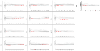
Sliceplorer evaluation results
Filter
With filter we want to essentially do isosurface filtering. Is the function ever above a particular value and if so, when?
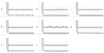
Click on the tabs below to see examples of the different datasets viewed with the different techniques. The individual images can be clicked for a larger version.


Solution descriptions
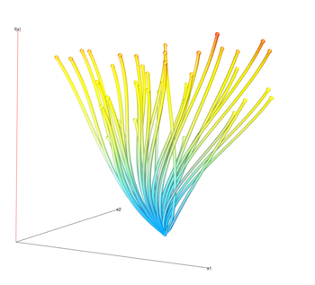
Gerber et al.
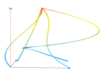
This is essentially a direct visualizaiton of the Morse-Smale complex. We could try to estimate the size of the parameter space above or below a certain value by estimating the area covered by the graph. The lines that connect the critical points in the graph are estimations of the curvature of the function under examination. Furthermore, the x-axes in the plot do not have any direct coorespondence with the input parameter space. It would be difficult to estimate the area covered above a certain y-value let alone recover the input values that correspond to this.
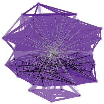
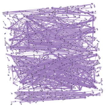
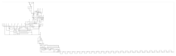
Contour tree
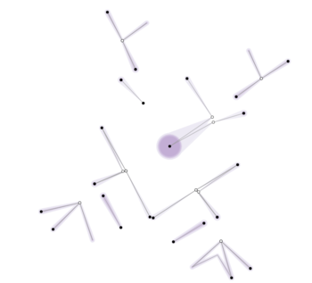
The graph layout algorithm tries to lay out the tree so that the y-position of the nodes relates to the function value. The contour tree only shows extrema and saddle points so these are the only points possible for which we can find the function value. In order to get some sense of what function values are over a particular value we first find the node with that value in the tree. Then we can estimate the proportion of input values above this value by the proportion of nodes that are above the one chosen.
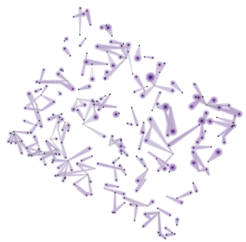
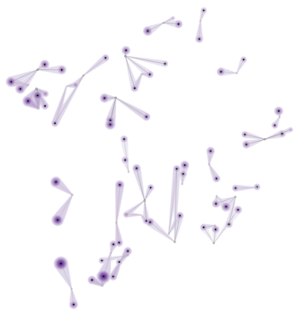
Topological spine
The concentric rings around each extrema are colored proportional to the function value. Plus, the area is proportional to the area under the curve for that value. Therefore, this is supported in the topological spines technique.
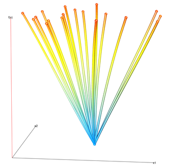
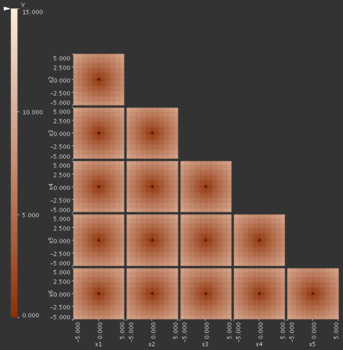
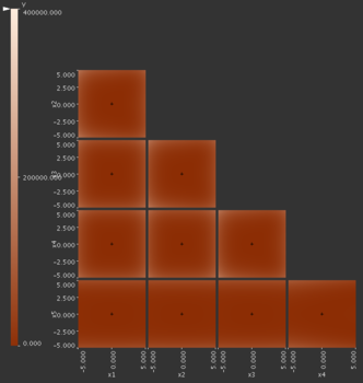
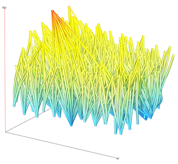
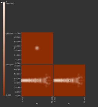
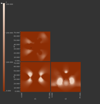
HyperSlice
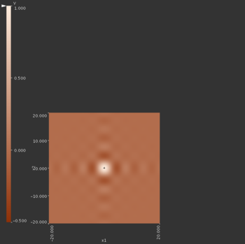
Given a particular focus point setting it is easy to find the parameter values that give a function value greater than some value by reading them off the heatmaps. The difficulty, however, comes with navigating the parameter space. If we want to know all parameter settings than we must carefully browse through all possible focus points. This is relatively easy in 3 dimensions since there is only one degree of freedom but in more it becomes very tedious and difficult.
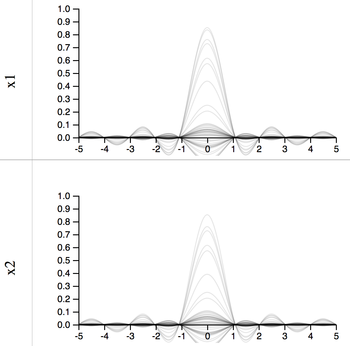
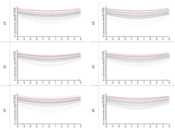
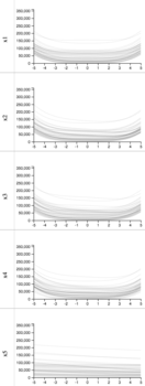
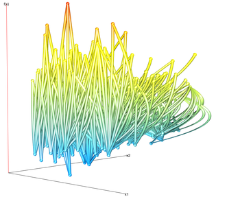
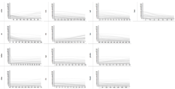
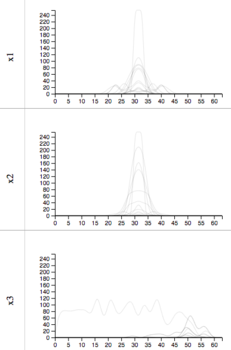
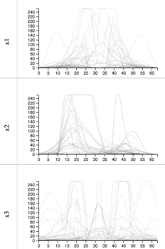
1D slices
With the slices view it is easy to see which slices are above a particular value. We find the portion of the slices that are above the y-value of interest. The user can highlight the slice to see what focus point and range of input will produce that output.