Sliceplorer evaluation results
Compute derived value
We want to visually derive summary statistics about the function under examination. What is the mean or variance of the function? Can we quantify (visually) which parameters have more effect than others on the function?
Click on the tabs below to see examples of the different datasets viewed with the different techniques. The individual images can be clicked for a larger version.
Solution descriptions
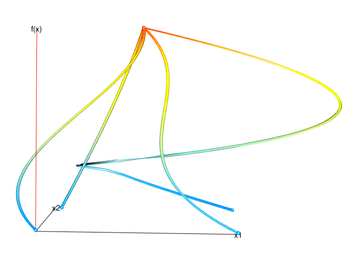
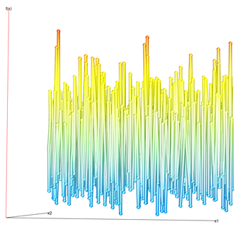
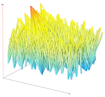
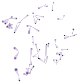
Gerber et al.
We can get a rough estimate of the variance of the function by looking at the pattern of extrema in the visualization. Due to the non-linear warping of the input space into two dimensions it is not possible to compute the “area under the curve” for a particular function value. This is required to visually derive measures such as the mean or sensitivity measures.
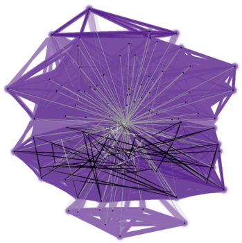
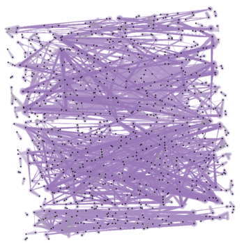
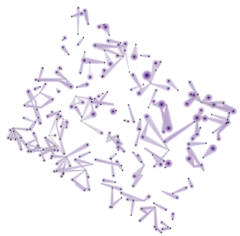
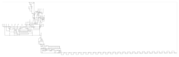
Contour tree
The graph layout algorithm tries to lay out the tree so that the y-position of the nodes relates to the function value. The contour tree only shows extrema and saddle points so these are the only points possible for which we can find the function value. We can get an idea for the range of possible output values of the function. However, since only the critical points are shown, any visual estimates of mean, variance, etc will only take into account critical points.
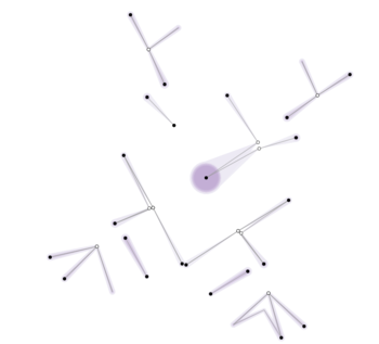
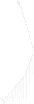
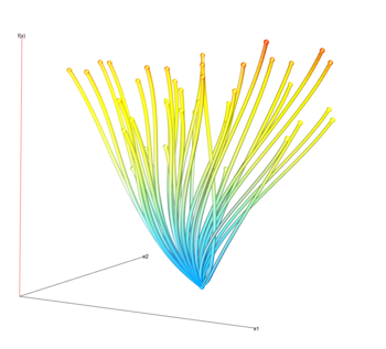
Topological spine
The concentric circles are related to the relative height (in function value) of the plots lets us examine the “peakiness” of certain extrema. However, metrics like the mean function value are very difficult to determine.
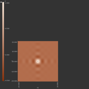
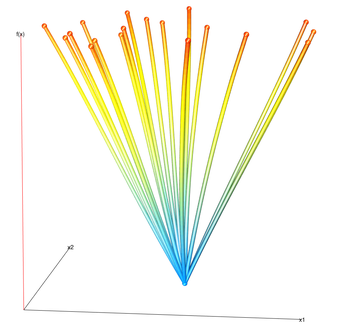
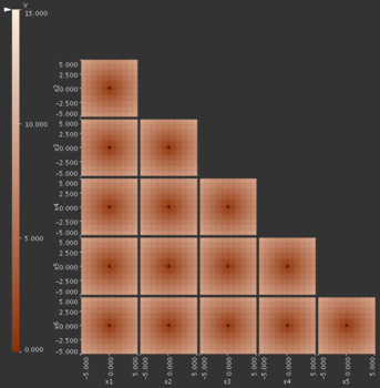
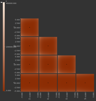
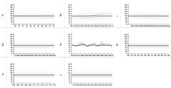
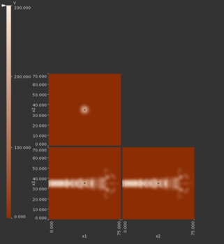
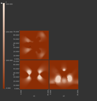
HyperSlice
In order to derive estimations of global statistics like mean and variance we need to carefully browse through all focus points to get a global view of the function. Local 1D and 2D sensitivity measures are easy to compute since we can look at the change in function value according to changes in parameter value.
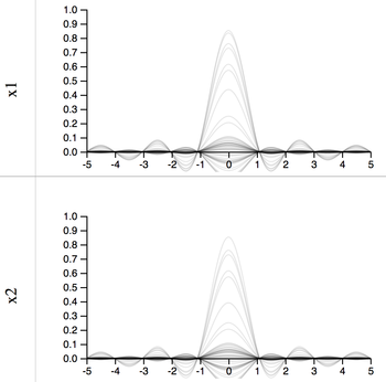
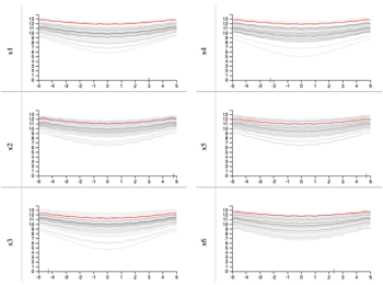
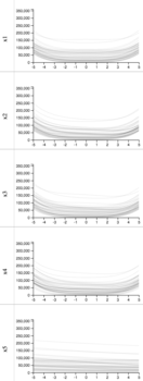
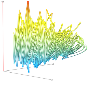
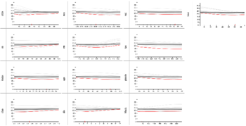
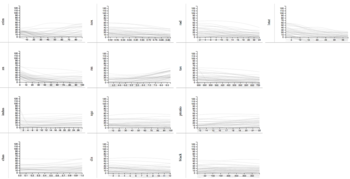
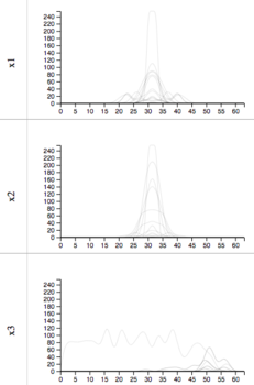
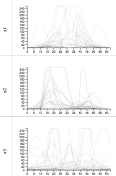
1D slices
The projections of slices allow the user to visually determine the distribution of slices. For example, the dark lines indicate that the average response value is that y value. We can also visually estimate the variance of the function by noting the wavinees of the lines.